What were the odds of Jack Dawson surviving the Titanic?

This article was originally published on Medium and can be found here

While browsing through the Kaggle, I noticed the famous Titanic dataset competition to predict which passengers would have survived. Having watched the American romance movie Titanic, it piqued my interest to find the extent to which the survival of passengers was dependent on age, gender, and social status.

Introduction to the chosen techniques

A decision tree is a decision support tool that uses a tree-like model of decisions and their possible consequences, including chance event outcomes, resource costs, and utility. — Wikipedia

Decision Trees help in understanding the data. Given their transparency and relatively low computational cost, Decision Trees are also useful for exploring the data before applying other algorithms. They help check the quality of engineered features and identify the most relevant ones by visualizing the resulting tree.

The main downsides of Decision Trees are their tendency to over-fit, inability to grasp relationships between features, and the use of greedy learning algorithms. Finding the best tree depth helps to resolve the issue of overfitting generally observed in such models.

Introduction of the dataset

Let’s load the data and get an overview. Data set can be found on here.

# Imports needed for the script
import numpy as np
import pandas as pd
import re
import xgboost as xgb
import seaborn as sns
import matplotlib.pyplot as plt
%matplotlib inline

import plotly.offline as py
py.init_notebook_mode(connected=True)
import plotly.graph_objs as go
import plotly.tools as tls

from sklearn import tree
from sklearn.metrics import accuracy_score
from sklearn.model_selection import KFold
from sklearn.model_selection import cross_val_score
from IPython.display import Image as PImage
from subprocess import check_call
from PIL import Image, ImageDraw, ImageFont
from sklearn.preprocessing import LabelEncoder
from sklearn_pandas import DataFrameMapper
from sklearn.preprocessing import OneHotEncoder

# Loading the data
train = pd.read_csv('train.csv')
test = pd.read_csv('test.csv')

# Showing overview of the train dataset
train.head(5)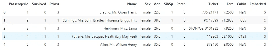

#Check the dimensions of the dataset
train.shape

# Check for null values in train and test data
print("Null values in the train data - ")
display(train.isnull().sum())

print("\nNull values in the test data - ")
display(test.isnull().sum())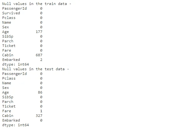

def concat_df(train, test):
    return pd.concat([train, test], sort = True).reset_index(drop=True)

full_data_df = concat_df(train, test)

#Check the percentage of missing data in entire data for column Age and Cabin
print("Percentage of missing values for age variable in entire data - ")
display(round(full_data_df['Age'].isnull().sum()/len(full_data_df)*100.0))

print("\nPercentage of missing values for cabin variable in entire data - ")
display(round(full_data_df['Cabin'].isnull().sum()/len(full_data_df)*100.0))

The dataset consists of 891 rows and 12 columns:

1. PassengerId

2. Survived: Only present in train dataset and is already in binary format

   0 = No
   1 = Yes

3. Pclass: A proxy for socio-economic status (SES)

   1st = Upper
   2nd = Middle
   3rd = Lower 

4. Name

5. Sex

6. Age: Fractional if less than 1. If the age is estimated, it is in the form of xx.5. Null values are observed in train and test data. 20% of data is missing in the entire dataset

7. Sib Sp: The dataset defines family relations

   Sibling = brother, sister, stepbrother, stepsister
   Spouse = husband, wife (mistresses and fiancés were ignored)

8. Parch: The dataset defines family relations

   Parent = mother, father
   Child = daughter, son, stepdaughter, stepson
   *Some children traveled only with a nanny, therefore parch=0

9. Ticket: Have many unique values with numbers and text

10. Fare: Null value observed in test data

11. Cabin: Null values observed in train and test data. 77% of data is missing in the entire dataset

12. Embarked: Port of Embarkation

    C = Cherbourg
    Q = Queenstown
    S = Southampton

Null value observed in train data

Input encoding/input representation (How and why?)

Dealing with missing values as observed in “Introduction of the dataset”

Age

plt.hist(train.Age, edgecolor='black')
plt.xlabel('Age')
plt.ylabel('count')
plt.show()

As observed in the above section 20% of the age variable is missing in the entire data set. However, one hypothesis is that age played a vital role in the survival of passengers. Hence instead of deleting the rows with missing values, the median should be a good choice for substitution based on the right-skewed distribution of the age graph.

One hypothesis is that the median age differs for the passenger classes and sex.

#Check whether the thesis holds true
display(train.groupby(['Pclass', 'Sex'])['Age'].median())

The hypothesis may be true as passengers with higher socioeconomic status are older on average which can be attributed to the generalization that older people would have advanced further in their professional careers. At the same time, there is a uniform pattern for median difference for sex. Females tend to be younger.

Hence, median values are used for age based on the “Pclass” and “Sex” variables

full_data_df['Age'] = full_data_df.groupby(['Pclass', 'Sex'])['Age'].apply(lambda x: x.fillna(x.median()))

Fare

full_data_df.loc[full_data_df['Fare'].isnull()]

There is one missing fare value in the whole data set. Mr. Thomas was in passenger class 3, traveled alone, and embarked in Southampton. We will take other cases from people in this category and replace the missing Fare with the median of this group.

passenger_1043 = full_data_df[(full_data_df['Pclass']==3) & (full_data_df['SibSp'] == 0) & (full_data_df['Embarked'] == 'S')]['Fare'].median()
full_data_df.loc[full_data_df['Fare'].isnull(), 'Fare'] = passenger_1043
print(passenger_1043)

7.925 --> Median Fare

Embarked

full_data_df.loc[full_data_df['Embarked'].isnull()]

For train dataset, there are only 2 missing values. We can simply input the mode or apply a similar procedure as that of fare. However, quick research on Google engine led us to https://www.encyclopedia-titanica.org/titanic-survivor/ which showed both of them embarking from Southampton.

full_data_df.loc[full_data_df['Embarked'].isnull(), 'Embarked'] = 'S'

All the missing values are dealt with for variables “age”, “fare” and “embarked”. For now, “cabin” variable is ignored as missing data is 77% in the entire dataset.

display(full_data_df.isnull().sum())

##Feature Engineering

Creating new feature

Title

full_data_df['Title'] = full_data_df.Name.str.extract(r'([A-Za-z]+)\.', expand=False)
full_data_df.Title.value_counts()

There are 18 different titles in our data set.

The common titles are (Mr/Miss/Mrs/Master). Some of the titles (Ms/Lady/Sir) can be grouped into common titles.

The remaining unclassified titles, with less than 10 cases will be assigned to the category “others”.

full_data_df['Title'].replace(['Ms', 'Mlle', 'Mme'], 'Miss', inplace=True)
full_data_df['Title'].replace(['Lady'], 'Mrs', inplace=True)
full_data_df['Title'].replace(['Sir', 'Rev'], 'Mr', inplace=True)

common_title = (full_data_df['Title'].value_counts() < 10)
full_data_df['Title'] = full_data_df['Title'].apply(lambda x: 'Others' if common_title.loc[x] == True else x)
full_data_df.groupby('Title')['Title'].count()

Family Size

SibSp defines how many siblings and spouses a passenger had and parch how many parents and children. We can summarize these variables into the family size.

#add one to include the passenger itself
full_data_df['FamilySize']= full_data_df['SibSp'] + full_data_df['Parch'] + 1

Binning

Binning is a way to group several more or less continuous values into a smaller number of “bins”. It makes the model more robust and avoids over-fitting.

Age

full_data_df.boxplot(column=['Age'], figsize=(7,7))

With cut, the bins are formed based on the values of the Age variable, regardless of how many cases fall into a category. This is done so that the outliers do not irritate the algorithm.

full_data_df['Age'] = pd.cut(full_data_df['Age'].astype(int),  5)
full_data_df['Age'].value_counts()

#Encoding the bins into number for modelling
label = LabelEncoder()
full_data_df['Age'] = label.fit_transform(full_data_df['Age'])full_data_df['Age'].value_counts()

Fare

full_data_df.boxplot(column=['Fare'], figsize=(7,7))

The range of values is much higher for fare compared to age. With qcut we decompose Fare distribution so that there is the same number of cases in each category/bin.

full_data_df['Fare'] = pd.qcut(full_data_df['Fare'],  5)
full_data_df['Fare'].value_counts()

#Encoding the bins into number for modelling
full_data_df['Fare'] = label.fit_transform(full_data_df['Fare'])full_data_df['Age'].value_counts()

Labeling and One Hot Encoding

Label Encoding maps non-numerical values to numbers. This is because most algorithms cannot do anything with strings, so the variables are often recoded before modeling.

A one-hot encoding is a representation of categorical variables as binary vectors. This first requires that the categorical values be mapped to integer values. Then, each integer value is represented as a binary vector that is all zero values except the index of the integer, which is marked with a 1.

Many algorithms assume that there is a logical sequence within a column. However, this is not always expressed by the numerical ratio. Therefore it is needed to one-hot encoding the variables afterward.

#Labeling
non_numeric_variables = ['Embarked', 'Sex', 'Title']

for variable in non_numeric_variables:
  full_data_df[variable] = label.fit_transform(full_data_df[variable])
  
#One hot Encoding
variables = ['Pclass', 'Sex', 'Embarked', 'Title', 'FamilySize', 'Age', 'Fare']

encoded_variables = []

for variable in variables:
  encoded_feature = OneHotEncoder().fit_transform(full_data_df[variable].values.reshape(-1, 1)).toarray()
  num = full_data_df[variable].nunique()
  cols = ['{}_{}'.format(variable, num) for num in range(1, num + 1)]
  encoded_df = pd.DataFrame(encoded_feature, columns=cols)
  encoded_df.index = full_data_df.index
  encoded_variables.append(encoded_df)

full_data_df = pd.concat([full_data_df, *encoded_variables], axis=1)
full_data_df.head(2)

Coding for the implementation

Split the dataset into train and test data

def divide_df(full_data_df):
  return full_data_df.loc[:890], full_data_df.loc[891:].drop(['Survived'], axis=1)


train_data, test_data = divide_df(full_data_df)

Drop columns for which new columns are created through one hot encoding and redundant columns like cabin, passengerid, name, etc.

drop_cols_train = ['Embarked', 'FamilySize', 'Age','Fare' ,'Name','Parch', 'PassengerId', 'Pclass', 'Sex', 'SibSp', 'Title', 'Ticket', 'Cabin']
train_data = train_data.drop(columns=drop_cols)
test_data = test_data.drop(columns=drop_cols)

Finding an optimal depth by cross validation method to avoid overfitting

cross_validation_folds = KFold(n_splits=10)
accuracies = list()
max_attributes = len(list(test_data))
depth_range = range(1, max_attributes + 1)

# Testing max_depths from 1 to max attributes
for depth in depth_range:
    fold_accuracy = []
    tree_model = tree.DecisionTreeClassifier(max_depth = depth)
    for train_fold, valid_fold in cross_validation_folds.split(train_data):
        f_train = train_data.loc[train_fold]
        f_valid = train_data.loc[valid_fold]

        model = tree_model.fit(X = f_train.drop(['Survived'], axis=1), y = f_train["Survived"])
        valid_acc = model.score(X = f_valid.drop(['Survived'], axis=1), y = f_valid["Survived"])
        fold_accuracy.append(valid_acc)

    avg = sum(fold_accuracy)/len(fold_accuracy)
    accuracies.append(avg)
    
df = pd.DataFrame({"Max Depth": depth_range, "Average Accuracy": accuracies})
df = df[["Max Depth", "Average Accuracy"]]
print(df.to_string(index=False))

The best max_depth parameter seems therefore to be 5 which has 82.82% average accuracy across the 32 folds)

Hence, 5 is used as the max_depth parameter for the final model.

# Create arrays of train, test and target dataframes to feed into our models
y_train = train_data['Survived']
x_train = train_data.drop(['Survived'], axis=1).values 
x_test = test_data.values

# Create Decision Tree with max_depth = 5
decision_tree = tree.DecisionTreeClassifier(max_depth = 5)
decision_tree.fit(x_train, y_train)

# Export our trained model as a .dot file
with open("tree.dot", 'w') as f:
     f = tree.export_graphviz(decision_tree,
                              out_file=f,
                              max_depth = 5,
                              impurity = True,
                              feature_names = list(train_data.drop(['Survived'], axis=1)),
                              class_names = ['Died', 'Survived'],
                              rounded = True,
                              filled= True )
        
#Convert .dot to .png to display
check_call(['dot','-Tpng','tree.dot','-o','tree.png'])

img = Image.open("tree.png")
draw = ImageDraw.Draw(img)
draw.text((10, 0), (0,0,255))
img.save('sample-out.png')
PImage("sample-out.png")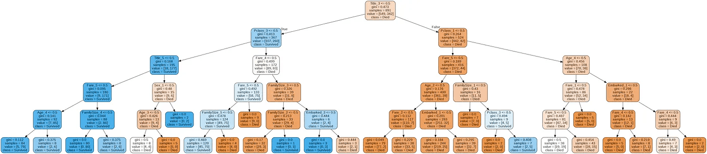

decision_tree_accuracy = round(decision_tree.score(x_train, y_train) * 100, 2)
decision_tree_accuracy

#Decision Tree Accuracy
84.18

Analysis of Results

The decision tree achieved an accuracy of 84.18% across the training dataset.

Graphical Tree Representation:

1. The first line of each node except the leaf node shows the splitting condition in the form “feature <= value”.
2. Next Gini Impurity of the node, is a measurement used to build Decision Trees to determine how the features of a dataset should split nodes to form the tree
3. Samples is the number of observations contained in the node.
4. Value shows the class distribution of the samples [died count, survived count].
5. Class corresponds to the predominant class of each node

Dictionary of labels:

1. {‘Master’: Title_1, ‘Miss’: Title_2, ‘Mr’: Title_3, ‘Mrs’: Title_4, ‘Others’: Title_5}
2. {1: Pclass_1, 2: Pclass_2, 3: Pclass_3}
3. {Female: Sex_1, Male: Sex_2}
4. Age and Fare have been mentioned above

Model can be summarized with following rules:

• If it doesn’t include “Mr” Title, and Passenger class is not 3rd class, then we classify it as survived. (all the branches on the left side of the tree lead to a blue node)
• If our observation includes “Mr” Title, and Passenger class is not 1st class then we classify it as not survived (has the highest casualties. Out of the 549 casualties in test data, 372 casualties belong to this class)
• If our observation belongs to age bracket of 16 and above and has “Mr” title then the mortality rate increases

With the same observation if we consider Jack Dawson from Titanic movie, age 20 years, a poor artist, based on the above rules he fell right into the class of non-survivals.

A strong correlation can be observed with respect to survival and gender, age & social status class.